Experimental Uncertainty

Xiaoping Du

Department of Mechanical and Aerospace Engineering

Missouri University of Science and Technology

February 8, 2014

1. Introduction

Experiments require taking measurements of physical quantities, such as velocity, time, and voltage. We generally assume that the “true” values of the quantities to be measured exist if we had a perfect measuring apparatus and followed a perfect procedure. The measurements, however, are always subject to unavoidable uncertainty due to the limitations of the measuring apparatus, random environment, and even fluctuations in the value of the quantity being measured.

As uncertainty is an unavoidable part of the measurement process, we should at first identify its sources and effects, and then quantify and report it. We should also seek to reduce measurement uncertainty whenever possible.

The result of any measurement has two components as shown in the following expression for a measured temperature.

The first term on the right-hand side is a numerical value that gives the best estimate of the quantity measured, and the second term indicates the degree of uncertainty associated with the estimated value. This result tells that the temperature measured is most likely to be 20°C, but it could be between 19°C and 21°C. In this chapter we study how to get the expression as the one in Eq. (1) for a quantity measured.

The other task of this chapter is uncertainty propagation. If the measured quality, for example, the temperature T in Eq. (1), is used as an input variable for an analysis, the analysis result for the output variable will also be naturally reported in the same form as Eq. (1), having the best estimate of and the associated uncertainty term. The second term is the result of the uncertainty in T propagated to . The task of uncertainty propagation is to find both of the two terms of .

2. Experimental Errors

In this section, we discuss experimental errors and their types.

2.1 Experimental errors

Experimental error is the difference between the true value of the parameter being measured and the measured value. The error of a measurement is never exact because the true value is never exactly known. Measurement errors could be either positive or negative.

A measurement error can be assessed by its accuracy and precision.

Accuracy measures how close a measured value is to the true value. As discussed above, the true value may never be exactly known, and it is difficult or even impossible to determine the accuracy of a measurement.

Precision measures how closely two or more repeated measurements agree with each other. Good repeatability means higher precision.

The distinction between accuracy and precision is illustrated in Fig.1.

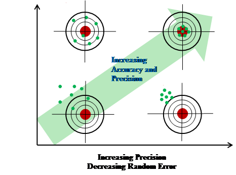
Fig. 1 Accuracy and Precision

Generally speaking, the accuracy and precision can be increased by decreasing the systematic and random errors, respectively. These two errors constitute the experimental error. Next we discuss the two types of error.

2.2 Systematic errors

Systematic errors are those that affect the accuracy of a measurement. Systematic errors are not determined by chance but are introduced by an inaccuracy inherent in a measuring instrument or measuring process. In other words, systematic errors may occur because of something wrong with the instrument or its data handling system or because of the wrong use of the instrument. In the absence of other types of errors, systematic errors yield results systematically in repeated measurements, either greater than or less than the true value. In this sense, systematic errors are “one-sided” errors.

For example, you use a cloth tape measure to measure the length of a table. The tape measure has been stretched out from a number years of use. As a result, your length measurements will always be shorter than the actual length.

If a systematic error is known to be present in the measurement, you should either to correct it or report it in your uncertainty statement. It is, however, hard to detect or reduce systematic errors. Below are some general guidelines.

· Calibrate the measuring instrument if the systematic error comes from poor calibration.

· Compare experimental results from your instrument with those from a more accurate instrument so that you have a good idea about how large systematic error of your instrument is.

· Change the environment, which interferes with the measurement process, so that the accuracy of the measuring instrument is highest.

2.3 Random experimental errors

Random errors are errors affecting the precision of a measurement. Random errors can be easily detected by different observations from repeated measurements. Random errors are commonly form unpredictable variations in the experimental conditions under which the experiment is performed. For example, random errors can come from electric fluctuations within components used in a measuring instrument or variations in temperature change in a lengthy experiment.

In the absence of other types of errors, repeated measurements yield results fluctuating above and below the true value or the average of the measurements. This indicates that random errors are “two-sided” errors.

3. Experimental Uncertainty Quantification

As shown in the expression in Eq. (1), when reporting the experimental result, we have the best estimate term () and the uncertainty term (). In this section, we focus on using statistical techniques to find both of the terms.

Uncertainty herein is a quantification of the double about the measurement result. Uncertainty quantification provides us with an estimate of the limits to which we can expect an error to go as shown in Eq. (1).

Suppose a quantity to be measured is X, and its measurements are ,,…, , where N is the number of repeated measurements.

With the N measurements, the obvious question we may ask is: “What is the best estimate of X?” If the only error source is from random fluctuations, given that the random error is a “two-sided” error, a nature answer is to use the average of the measurements. Averaging the measurements makes the fluctuations on both sides cancelled out to some degree.

The average or mean is calculated by

After obtaining the best estimate term, we now look at the uncertainty term. The uncertainty in the set of the measurements ,,…, can be quantified by the degree of scatter of the measurements around the mean.

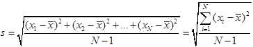
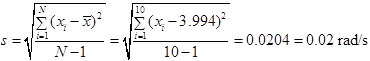
The most commonly used measure of scatter is the sample standard deviation defined by

Example 1 A slider mechanism is show in Fig. 2. The motion input, which is the angular velocity of link AB, is measured. The ten measurements are given by rad/s. Determine the average and standard deviation of the measurements.

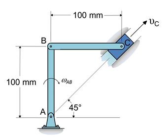
Fig. 2 Slider Mechanism

The average is given by

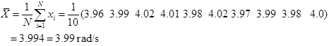
The average is considered the best estimate the angular velocity.

The standard deviation is computed by

Note that the number of significant digits used in the final result of the average (3.99 rad/s) is the same as the number of significant digits in the measurements. It does not make sense to use the calculated one (3.994 rad/s) because its last digit is beyond the precision of the measuring instrument.

After we have done the statistical analysis, we could state that the best estimate of is 3.99 rad/s. Of course, there is some degree of uncertainty because of the non-zero standard deviation. We should also report the associated uncertainty at a certainty confidence level. This requires us to know something about probability distributions. Next we discuss some basics about the normal distribution, which is the most commonly used distribution.

A normal distribution for random variable is determined by the mean and standard deviation of and is denoted by .

The probability density function (PDF) of , as shown in Fig. 3, tells us everything about , especially the likelihood of the occurrence of certain possible values of . It is easy to see that the values around the mean have the highest chance to occur. Fig. 3 also indicates that the range defined by covers about 95% possible values of . In other words, the probability that the actual values of fall into the interval is about 95%.

If we report our experimental result in the form of , we expect that the true value that was measured has a 95% chance to reside in . We can then define the uncertainty term as

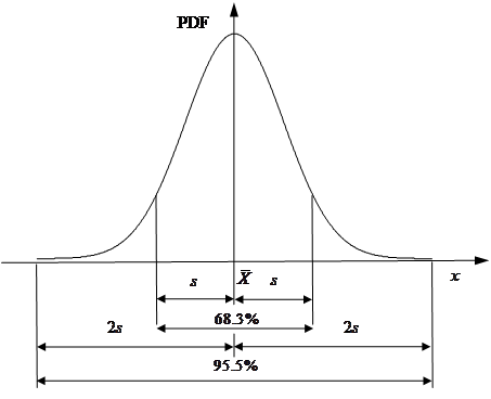
Fig. 3. PDF of a normal random variable

Example 2 The angular velocity of link AB of the mechanism shown in Fig. 2 is measured, and the ten measurements are given in Example 1. Report the measurement result in a standard form.

In Example 1, we have obtained the average and the standard deviation . The uncertainty term is then

Using the same number of significant figures as , we have

The measurement result is then stated as

With the result, we expect that the chance of the true angular velocity being within is 95%.

4. Combined Uncertainty

In the last example, uncertain comes from only one source. If uncertainty is from multiple independent sources, we should combine their effects by using the following equations.

Assume that random variables and are independent and that their standard deviation are and , respectively. The standard deviation of is then given by

Then the combined uncertainty term is

Let the uncertainty terms associated with and be and , respectively. The combined uncertainty term can then be rewritten as

or

We can generalize the result to a general case with

Example 3 The angular velocity of link AB of the mechanism shown in Fig. 2 is measured, and the ten measurements are given in Example 1. The measuring equipment manufacturer claims an accuracy of on the equipment readout. This accuracy is assumed at 95% confidence. Estimate the overall measurement uncertainty and report the measurement result in the standard notation.

There are two sources of uncertainty. We have found the uncertainty term from random fluctuations in Example 2. The other source of error is from the measuring instrument itself with . According to Eq. (11), the combined overall uncertainty term is

Then the measurement result is stated as

5. Uncertainty Propagation

Measured quantities may be used for an analysis. Let the measured quantities be and the output of the analysis be . Also assume . From experiments, we have .

Uncertainties in will be propagated to through . Our task is to find .

We start pour discussions from a linear function.

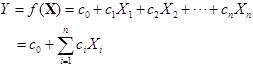
where is constant.

If are independent, we have

where is the average of .

The standard deviation of is

where is the standard deviation of , and .

Since , we obtain

We now look at the general case where is a nonlinear function. To use the results we have obtained for a linear function, we linearize at the means of , as

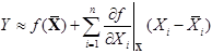
where and are all constant. We then have

and

where .

The uncertainty term for is the same as given in eq. (15).

Example 4 The angular velocity of link AB of the mechanism shown in Fig. 2 (The figure is redrawn in Fig.4 for convenience) is measured, and ten measurements are given in Example 1. The measuring equipment manufacturer claims an accuracy of on the equipment readout. This accuracy is assumed at 95% confidence. The measured value of the length of link AB is . Determine the velocity of the slider , and state the result in the standard notation.

Fig. 4 Slider Mechanism

Let and . Then and . The result was obtained from Example 3. and .

We now perform kinematics analysis to find . The function for is given by

The velocity of the slider is then reported as

6. Conclusions

The measurement error is the difference between the quantity being measured and its true value. The measurement error consists of systematic error and random error. The measurement error can be characterized by uncertainty analysis, and the measurement results is commonly stated in the form of , where is the best estimate (usually the average of repeated measurements), and is the uncertainty term with a stated confidence level (usually 95%).

When a measured quantity is used in an analysis, the effect of the uncertainty in the measurement quantity on the analysis result can be quantified through uncertainty propagation, which is often based on the first order Taylor expansion.