Reliability-Based Design (RBD)
A
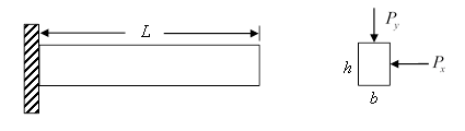
cantilever beam is subjected to two random forces ![]() lb and
lb and ![]() N at the tip as shown. The yield stress is
N at the tip as shown. The yield stress is
![]() psi, the Young’s Modulus is
psi, the Young’s Modulus is ![]() psi, and the allowable deflection is
psi, and the allowable deflection is ![]() in. The length of the beam is a random
variable with
in. The length of the beam is a random
variable with ![]() in. Given the minimum probabilities of
in. Given the minimum probabilities of ![]() for failure modes of excessive normal
stress and excessive deflection, find the optimal solution so that the volume
of the beam is minimized. The ranges of the beam size are given by
for failure modes of excessive normal
stress and excessive deflection, find the optimal solution so that the volume
of the beam is minimized. The ranges of the beam size are given by ![]() and
and ![]() .
.
Solution
The design variable are ![]() and
and ![]() ; the objective function is
; the objective function is ![]() . The random parameters are
. The random parameters are ![]() . There are two failure modes. For the
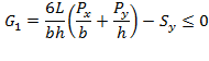
failure mode of excessive stress, the limit-state function is given by
. There are two failure modes. For the
failure mode of excessive stress, the limit-state function is given by
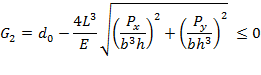
For the failure mode of excessive deflection, the limit-state function is given by
All the information we know are listed below.
![]() lb
lb
![]() lb
lb
![]()
![]() psi
psi
![]() in
in
![]() in
in
![]() ,
,![]() ,
,![]()
![]() = 0.999, or
= 0.999, or ![]()
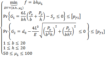
In order to find the optimal solution, we minimize ![]() with two reliability constraints. The
optimization model is given by
with two reliability constraints. The
optimization model is given by
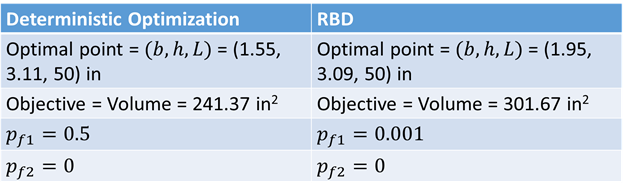
The First Order Second Moment method (FOSM) is used for reliability analysis, and Matlab is used to solve the optimization model. The optimal solution is as follows:
Design variables: ![]()
Objective function: ![]()
Probability of failure for failure mode 1: ![]()
Probability of failure for failure mode 2: ![]()
The compare RBD with deterministic optimization (only mean values are used), we give the results from both methods in the following table.
The Matlab codes are given below.
1) Main function
% Main program of RDB for a cantilever beam
% Xiaoping Du, Missouri S&T, 04/10/2017
clear all; warning off;
%----------------------- Reliability-Based Design---------------
dv0 = [2.0,3.0,40.0]; % dvs=[b,h,uL]
dvl = [1.0,1.0,50.0]; % lower bounds of dvs
dvu = [20.0,20.0,100.0]; % upper bounds of dvs
required_pf(1:2) = 0.001; % Required probabilities of failure
options = optimset('Display','iter','MaxFunEvals',1000); % Display convergence history
dv = fmincon('rbd_obj_fun',dv0,[],[],[],[],dvl,dvu,'rbd_con_fun',options,required_pf);
%obj_fun: function for objective
%con_fun: function for constraints
%Posterior analysis
obj = rbd_obj_fun(dv);
[g,ceq] = rbd_con_fun(dv,required_pf); %g=pf-required_pf
pf = g+required_pf;
%Display the results
disp('------------------RBD Results-------------------');
disp(['The optimal point = ',num2str(dv)]);
disp (['The objective function = ',num2str(obj)]);
for i = 1:2
disp(['Probability of failure mode ',num2str(i),' = ',...
num2str(pf(i))]);
end
2) Objective function
%Objective function
function f = rbd_obj_fun(dv,required_pf)
%dvs=[b,h,uL]
f = dv(1)*dv(2)*dv(3); %Volume
3) Constraint function
% Constraint functions
% FOSM is used to calculate the probability of failure
function [g,ceq] = rbd_con_fun(dv,required_pf)
ceq = []; %No equality constraints
%d=(b,h), X=(L), P=(Px,Py,S,E)
%dv=[b,h,uL];
b = dv(1); h = dv(2); L = dv(3);
Px = 500; Py = 1000; S = 4.0e4; E = 29.0e6; %Mean
sL = 0.1; sPx = 100; sPy = 100; sS = 2.0e3; sE = 3.0e6; %Std
%Calculate mean of g
ug1 = S-6*L/b/h*(Px/b+Py/h);
ug2 = 2.5-4*L^3/E*((Px/b^3/h)^2+(Py/b/h^3)^2)^0.5;
%Calculate std of g
dg1dL = 6/b/h*(Px/b+Py/h);
dg1dPx = 6*L/b/h/b;
dg1dPy = 6*L/b/h/h;
dg1dE = 0;
dg1dS = 1;
dg2dL = -12*L^2/E*(Px^2/b^6/h^2+Py^2/b^2/h^6)^(1/2);
dg2dPx = -4*L^3/E/(Px^2/b^6/h^2+Py^2/b^2/h^6)^(1/2)*Px/b^6/h^2;
dg2dPy = -4*L^3/E/(Px^2/b^6/h^2+Py^2/b^2/h^6)^(1/2)*Py/b^2/h^6;
dg2dE = 4*L^3/E^2*(Px^2/b^6/h^2+Py^2/b^2/h^6)^(1/2);
dg2dS = 0;
stdg1 = ((dg1dL*sL)^2+(dg1dPx*sPx)^2+(dg1dPy*sPy)^2+(dg1dE*sE)^2+(dg1dS*sS)^2)^0.5;
stdg2 = ((dg2dL*sL)^2+(dg2dPx*sPx)^2+(dg2dPy*sPy)^2+(dg2dE*sE)^2+(dg2dS*sS)^2)^0.5;
%Calculate reliability
pf(1) = normcdf(-ug1/stdg1);
pf(2) = normcdf(-ug2/stdg2);
%Constraints
g(1) = pf(1)-required_pf(1); %Matlab uses g<=0
g(2) = pf(2)-required_pf(2);